Why the Kelpie ORT coincidence background is a triangle
Note on the clock. This document is written for the 10 MHz reference clock, where the oscillator period
Pis 100 ns.Pis one period of the reference clock, so it is 20 ns at 50 MHz, 200 ns at 5 MHz and 500 ns at 2 MHz, and the triangle's base, the CAR penaltyT/Pand the number of folded cycles all move with it. Every formula below is in terms ofP; only the numbers assume 100 ns. In code, passopen_shutter_time_s(orfull_scale_s) — nothing assumes 100 ns any more.
TL;DR — The Kelpie ORT timestamp records only where in a 100 ns oscillator cycle a photon arrived, not which cycle inside the ~9 µs frame. That single fact — losing the absolute timestamp and keeping only the phase — turns the flat accidental background of a normal time‑tagger into a triangle, and concentrates the accidentals under the peak by a factor T_frame / T_phase ≈ 9 µs / 100 ns ≈ 90. It is not an analysis bug; it is a direct consequence of folding 9 µs into 100 ns.
1. Two ways to timestamp the same photon
Consider a photon that arrives at absolute time t inside one acquisition
frame of length T = 9 µs. The ring oscillator has period P = 100 ns, so we
can write
- Reference camera (absolute tagger). Stores the full
t(100 ps resolution over the whole frame). Bothkandφare kept. - Kelpie ORT. Stores only
φ— the phase within the current 100 ns cycle — and only one value per pixel per frame. The cycle indexkis thrown away.
Everything below follows from that one difference.
2. A coincidence is a difference of two timestamps
For a signal photon (pixel A) and an idler photon (pixel B) we histogram
- A true SPDC pair is simultaneous:
t_A = t_B(to within the ~100 ps jitter). ThenΔ = 0in both schemes — same cycle, same phase. The peak at Δ = 0 survives the folding. This is why you still see a peak. - An accidental pair is two independent photons. Their
Δdistribution is what changes shape — and that is the whole story.
3. The math: difference of two uniform times is a triangle
Photon arrival times within a frame are (to good approximation) uniform. Two independent uniform variables, differenced, give a triangular distribution — this is the autocorrelation of a boxcar:
If X, Y ~ Uniform(0, L) independently, then D = Y − X has density
a triangle peaking at D = 0, falling linearly to zero at |D| = L, with
Absolute tagger → base L = T
Absolute times are uniform over the whole frame, Uniform(0, T). So
accidentals form a triangle with base ±T = ±9 µs:
Over a normal ±ns coincidence window, that triangle is essentially flat and almost empty — the background you expect. (Left panel of the figure.)
Kelpie ORT → base L = P
Here is the key step. Taking a uniform time modulo the period,
maps Uniform(0, T) onto Uniform(0, P) exactly when T is a whole number
of periods (9000 = 90 × 100). Every one of the 90 cycles folds onto the same
[0, 100 ns) interval. So the phase is uniform on [0, P), and the accidental
difference φ_B − φ_A is a triangle with base ±P = ±100 ns:
4. The folding concentrates accidentals by T / P
Compare the accidental density right under the peak (at Δ = 0) in the two
schemes:
Folding 9 µs into 100 ns piles 90 frames' worth of accidental combinations on top of each other at Δ = 0. The number of true pairs at Δ = 0 is unchanged (they were already at 0). So the coincidence‑to‑accidental ratio drops by the same factor:
at the same singles rate, same resolution, same source.
The same thing in the time domain: aliasing pulls random Δ toward zero
Write any pair's true separation as
ORT records only the second term, Δ_rec = φ_B − φ_A, so
The discarded (k_B − k_A)·P — the global cycle offset — is the
absolute‑time information. Dropping it means:
- Random pairs are recorded with a shorter
|Δ|than they truly have. A random pair genuinely 3.5 µs apart (k_B − k_A = 35) is stored atΔ_rec = φ_B − φ_A ∈ (−100, +100) ns— it masquerades as a near‑coincidence. - And they cluster at zero, not spread flat. Because the two phases are each
uniform,
Δ_recis triangular — the aliasing preferentially yields small apparent separations, piling the fake near‑coincidences right under the true peak (density at 0 is 2× a flat spread of the same counts).
This is the physical content of the T/P concentration above: the long real
delta‑ts of random pairs — which on an absolute tagger form the flat,
out‑of‑the‑way background — are folded back onto Δ ≈ 0. True pairs already sit
at Δ = 0, so only the background moves onto the peak. The lost cycle
information does not just reduce contrast uniformly; it dumps the accidentals
exactly where they do the most damage.
5. Demonstration (same photons, two timestamps)
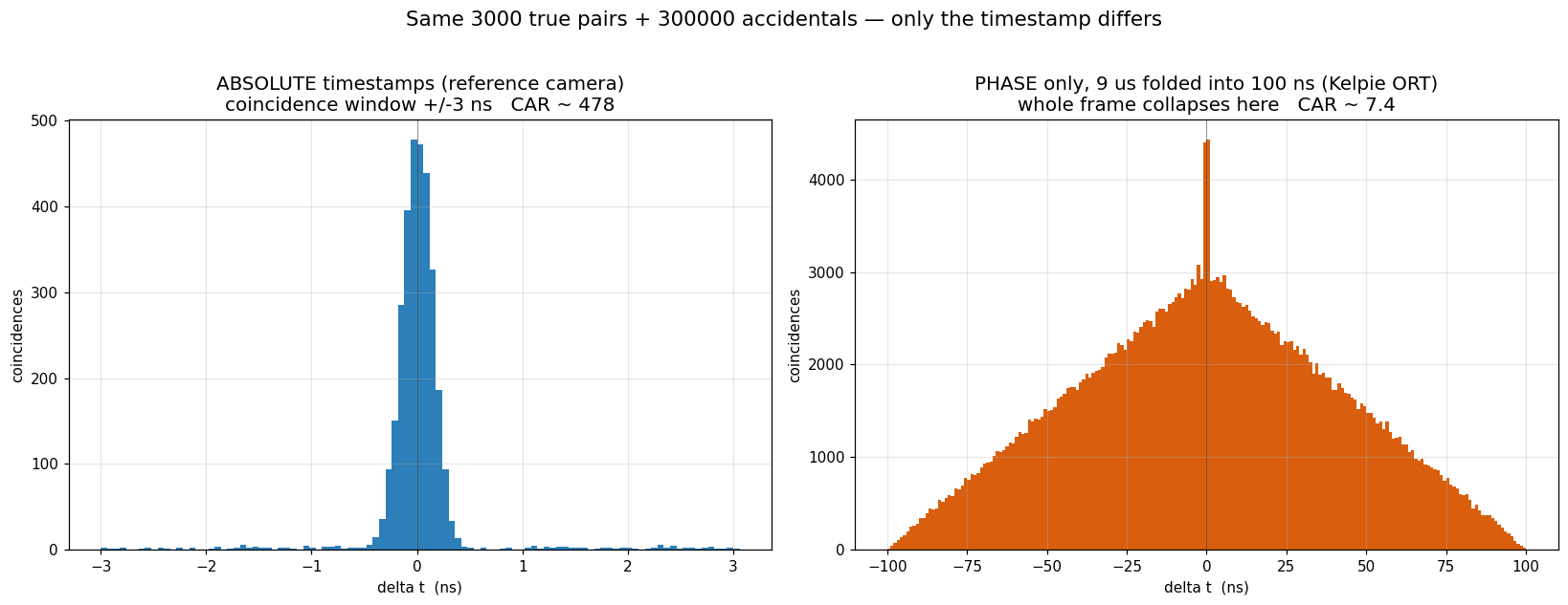
Both panels use the identical 3000 simultaneous pairs and 300 000 accidental pairs. Only the timestamp differs.
- Left — absolute timestamps: accidentals spread over ±9 µs, so in a ±3 ns window the background is flat and nearly empty; the peak dominates (CAR ≈ 480). This is your reference camera.
- Right — phase only (9 µs folded into 100 ns): every accidental collapses into the ±100 ns triangle; the peak is a thin spike on a large triangular pedestal (CAR ≈ 7). This is Kelpie ORT.
The real 2026‑07‑24 SPDC data reproduces the right panel exactly: a clean triangle from −100 ns to +100 ns with a sharp spike at 0.
6. Why this is not fixable in the analysis
The information that would flatten the background — the cycle index k, i.e. the
absolute time within the frame — was never recorded. Verified against the
MATLAB reference decoder (kelpie_data_ddr3.m): the timestamp field is only a
10‑bit coarse + 4‑bit fine value that wraps at P / 71.6 ps codes (~1397 at
10 MHz, ~6985 at 2 MHz; the field itself saturates at 8184 ≈ 586 ns), with no
counter for k. You cannot un‑fold a triangle back into a flat background
without k.
Two things also make it worse in practice:
- One timestamp per pixel per frame (first photon only): at high occupancy the true pair's photon is often preempted by an earlier uncorrelated photon, suppressing the peak on top of the concentrated background.
- Larger frames make it worse: the factor is
T/P, so a longerT(the DCR‑consistency check hintsTmay be ~40 µs, not 9 µs) means an even bigger triangle.
7. What restores it
Only recovering absolute time, or shrinking the fold:
| Lever | Effect on T/P |
Notes |
|---|---|---|
| Absolute / start‑stop timestamp mode | removes the fold entirely | needs firmware/HW support (a "stopped" TDC vs the free‑running one); memory notes a run failing because "the TDC never stopped", implying such a mode exists |
Shorter frame T |
linear improvement | T = 900 ns → 10× better CAR |
| Better focusing / more statistics | no change to CAR | improves count rate and significance, not contrast — still worth doing, just not a fix for the triangle |
8. Separate issue: peak width
The triangle explains the background shape and the contrast, but not the peak width (~500 ps measured vs ~100 ps expected). That is a timing‑ resolution question — code→time calibration (the flat ~71.6 ps/code is only an average; the density‑test LUT gives per‑code widths) and detector jitter — and is independent of everything in this document.